Bayesian Spatiotemporal Modelling of Relative AFP Reporting • spi

spi is an R package for identifying changes in non-polio acute flaccid paralysis (NPAFP) reporting relative to a district’s preceding reporting history. The surveillance performance index (SPI) compares reported NPAFP cases with the number expected, then compares the district’s observed-to-expected ratio with the corresponding national ratio. The package offers two ways to obtain the expected count. The simple SPI uses each district’s own earlier rate. The model-based SPI estimates it with a spatial and temporal model, which adds uncertainty intervals and monthly results.

SPI complements the conventional NPAFP rate. The NPAFP rate measures the absolute level of reporting, whereas SPI measures reporting relative to preceding reporting and the national pattern. A district can therefore continue to meet the NPAFP target while reporting substantially fewer cases than expected from its history. Conversely, a district with persistently low reporting can have an SPI near 1 while its NPAFP rate remains below the target. SPI should therefore be interpreted alongside the NPAFP rate, timeliness, specimen quality, and other surveillance information.

Installation

Install from GitHub:

# Install pak if needed
if (!requireNamespace("pak", quietly = TRUE)) install.packages("pak")
pak::pak("truenomad/spi")

The model-based functions, such as spi_expected() and spi_index(), need INLA, which is not on CRAN. spi_simple() needs neither INLA nor district boundaries. Install INLA with:

install.packages(
  "INLA",
  repos = c("https://cloud.r-project.org", "https://inla.r-inla-download.org/R/stable/")
)

Overview

For the simple SPI, start with annual NPAFP counts and under-15 population estimates by district. spi_simple() calculates annual SPI without INLA or district boundaries. For the model-based SPI, start with monthly NPAFP counts, annual under-15 population estimates, and district boundaries. spi_index() estimates expected counts with the spatial and temporal model and calculates annual or monthly SPI with credible intervals. The package also produces plots and maps, compares SPI with the conventional NPAFP target, and brings the results together for district review in the STEPS field guide.

Quick start

The bundled synth_surveillance data cover 236 districts in the fictional country Harad, from 2015 to 2024. All examples use synthetic data and require no access to GPEI POLIS.

library(spi)

synth <- synth_surveillance

The simple SPI

The simple SPI uses each district’s own earlier rate: expected cases = current population × earlier cases ÷ earlier child-years.

The figure works through the calculation for a hypothetical district.

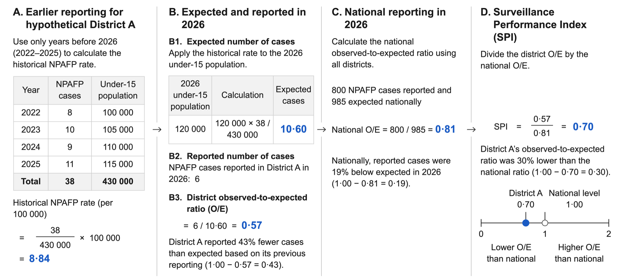
Worked simple SPI calculation for a hypothetical district: preceding cases and population give the historical rate, expected cases, the district and national observed-to-expected ratios, and the SPI

The simple SPI needs only annual counts and population by district. The bundled counts are monthly, so add them up to years first:

annual <- synth$cases |>
  dplyr::mutate(year = as.integer(format(month, "%Y"))) |>
  dplyr::summarise(count = sum(count), .by = c(adm2_guid, year))

Calculate annual SPI:

spi_simple_dy <- spi_simple(
  annual,
  population = synth$population,
  id_col = "adm2_guid",
  count_col = "count",
  pop_col = "pop_u15",
  first_assessment = 2018,
  verbose = FALSE
)

View the results:

spi_simple_dy$summary |>
  dplyr::select(adm2_guid, year, observed, expected, oe, spi, history_check) |>
  dplyr::slice_head(n = 6)
#> # A tibble: 6 x 7
#>   adm2_guid                     year observed expected    oe   spi history_check
#>   <chr>                        <int>    <dbl>    <dbl> <dbl> <dbl> <chr>        
#> 1 {01325AA0-BEA1-66FE-9B5C-88~  2018        2     1.08 1.86  1.69  ok           
#> 2 {040649D0-A0BA-C005-ADEF-90~  2018        7     6.74 1.04  0.946 ok           
#> 3 {04CBADAF-5577-E1AB-12F7-49~  2018       11    25.7  0.428 0.391 ok           
#> 4 {0673C3E5-5534-6578-70F4-B6~  2018       52    40.6  1.28  1.17  ok           
#> 5 {069B1B50-BB32-0C5A-DC20-C9~  2018        2     2.49 0.803 0.732 ok           
#> 6 {07BC4455-2DED-3E72-89F5-F1~  2018        4     9.65 0.415 0.378 ok

observed and expected are the reported and expected cases, oe is their ratio, and spi is that ratio divided by the national ratio for the year. spi_simple_explain() shows how one district’s value was calculated:

spi_simple_explain(
  spi_simple_dy,
  district = spi_simple_dy$summary$adm2_guid[1],
  year = 2023
)
#> 
#> -- District {01325AA0-BEA1-66FE-9B5C-88AA603382F3}, 2023 -----------------------
#> 
#> -- Current reporting --
#> 
#> Observed NPAFP cases                  1
#> Current population under 15     205 717
#> NPAFP rate                         0.49
#> 
#> -- Previous reporting --
#> 
#> Previous years                        8
#> Previous NPAFP cases                 16
#> Previous child-years          1 526 968
#> Previous rate                      1.05
#> 
#> -- Expected reporting --
#> 
#> Expected NPAFP cases               2.16
#> 
#> -- SPI --
#> 
#> District observed / expected       0.46
#> National observed / expected       1.14
#> SPI                                0.41
#> 
#> -- Data checks --
#> 
#> Population check                no flag

The simple SPI gives one value per district and year, without credible intervals. A district with no earlier year or no earlier NPAFP case has spi = NA; history_check records the reason. National centring uses only districts with positive expected counts. If those districts report no cases in the assessment year, the national ratio is zero and SPI is NA for every district.

With a table that has the columns district, year, npafp_cases and population_u15, spi_simple(afp_data) needs no other argument.

For the full simple SPI workflow, see Calculating the simple SPI.

The model-based SPI

Use the model-based SPI when you need credible intervals, monthly results, or more stable expected counts for districts with short or sparse reporting histories. spi_index() estimates each assessment year’s expected counts from the preceding years only, so it refits the model once per year. This example assesses 2018 to 2024 without covariates.

Calculate annual SPI, passing the district boundaries directly:

spi_dy <- spi_index(
  cases = synth$cases,
  population = synth$population,
  adjacency = synth$boundaries,
  first_assessment = 2018,
  id_col = "adm2_guid",
  n_draws = 500,
  seed = 42,
  verbose = FALSE
)

View the results:

spi_dy |>
  tibble::as_tibble() |>
  dplyr::select(adm2_guid, year, spi_median, spi_q05, spi_q95) |>
  dplyr::slice_head(n = 6)
#> # A tibble: 6 x 5
#>   adm2_guid                               year spi_median spi_q05 spi_q95
#>   <chr>                                  <dbl>      <dbl>   <dbl>   <dbl>
#> 1 {01325AA0-BEA1-66FE-9B5C-88AA603382F3}  2018      0.890   0.507   1.63 
#> 2 {01325AA0-BEA1-66FE-9B5C-88AA603382F3}  2019      2.00    1.16    3.38 
#> 3 {01325AA0-BEA1-66FE-9B5C-88AA603382F3}  2020      1.18    0.753   1.86 
#> 4 {01325AA0-BEA1-66FE-9B5C-88AA603382F3}  2021      1.09    0.758   1.65 
#> 5 {01325AA0-BEA1-66FE-9B5C-88AA603382F3}  2022      0.812   0.529   1.20 
#> 6 {01325AA0-BEA1-66FE-9B5C-88AA603382F3}  2023      0.369   0.259   0.531

spi_dy$national contains the national observed-to-expected ratio. Set centre = "none" for the uncentred district ratio. A district-year with no reported cases has an SPI of 0 and a 0 to 0 interval, because the interval reflects uncertainty in the expected count only; this is not certainty about surveillance performance.

For the full model-based SPI workflow, see Calculating the model-based SPI.

Recommended workflow

For the simple SPI:

Check the table with spi_check_inputs(method = "simple").
Calculate annual SPI with spi_simple().
Review history_check for missing SPI values and population_qc for population records to check.
Check the national observed-to-expected ratio.
Inspect individual districts with spi_simple_explain().
Compare SPI with the NPAFP target using spi_compare_npafp().

For the model-based SPI:

Check the inputs with spi_check_inputs().
Calculate annual SPI with spi_index(), which fits the expected-count model for each assessment year from the preceding years.
Compare SPI with the NPAFP target using spi_compare_npafp().
Check the credible intervals and the national observed-to-expected ratio.

Pass either comparison to spi_field_guide() to review districts using the STEPS components. For the simple SPI, the default cutoff is spi_cut = 0.5. This selects larger relative shortfalls for review; it does not measure uncertainty.

Learn more

The package website groups the articles as follows.

Using SPI:

Getting started with SPI: what SPI measures, how it differs from the NPAFP rate, and when to use the simple or model-based SPI.
Preparing data for SPI: prepare counts, population estimates, and district identifiers.
Using SPI with POLIS data: go from the POLIS AFP line list cleaned with polished to the simple and model-based SPI.
Interpreting SPI: understand SPI alongside the NPAFP rate, timeliness, and stool adequacy.
How SPI works: the simple and model-based calculations and their limitations.

Simple SPI:

Calculating the simple SPI: work through the annual calculation by hand, then with the package.

Model-based SPI:

Calculating the model-based SPI: fit the model and inspect outputs.
Model options and sensitivity: explore covariates, overdispersion, spatial structure, and sensitivity analyses.
Using SPI for district review: compare SPI with the NPAFP target, run the STEPS field guide, and produce district reports.

The function reference documents all exported functions.

Citation

To cite spi in publications, run citation("spi") in R, or use:

Yusuf, Mohamed A. and Nnanatu, Chibuzor Christopher (2026). spi: Bayesian Spatiotemporal Modelling of Relative AFP Reporting. R package version 0.3.0. https://doi.org/10.5281/zenodo.23008378

@Manual{spi,
  title  = {spi: Bayesian Spatiotemporal Modelling of Relative AFP Reporting},
  author = {Mohamed A. Yusuf and Chibuzor Christopher Nnanatu},
  year   = {2026},
  note   = {R package version 0.3.0},
  url    = {https://github.com/truenomad/spi},
  doi    = {10.5281/zenodo.23008378},
}

For users with POLIS access under a GPEI data-sharing agreement, polished retrieves and prepares data from the GPEI Polio Information System (POLIS) and calculates indicators such as the NPAFP rate, timeliness, and stool adequacy.

spi