
spi_index() estimates expected counts with a spatial and
temporal model fitted with INLA. It calculates annual or monthly SPI
with credible intervals. The model can give more stable expected counts
for districts with little reporting history by using information from
other districts. Getting started with
SPI compares the simple and model-based SPI, and Interpreting SPI explains the
results.
This article uses the bundled synthetic data to check inputs, calculate and plot SPI, and choose a reporting year that ends in a month other than December. The outputs shown here were computed with INLA when the article was built.
Input data
The model-based SPI needs three inputs, all using the same district ID column. Preparing data for SPI shows how to prepare them:
- monthly NPAFP case counts, one row per district and month;
- annual under-15 population, one row per district and year;
- district boundaries as an
sfobject.
If you have POLIS access under a GPEI data-sharing agreement, polished can retrieve and clean these inputs from POLIS.
The bundled synth_surveillance data cover 236 districts
in the fictional country Harad, from 2015 to 2024. The district ID
column is adm2_guid:
library(spi)
synth <- synth_surveillance

names(synth$cases)
#> [1] "adm2_guid" "month"     "count"
names(synth$population)
#> [1] "adm2_guid" "year"      "pop_u15"
names(synth$boundaries)
#> [1] "adm2_guid" "adm2_name" "adm1_name" "adm0_name" "geom"
month is the first day of each month, count
is the number of NPAFP cases reported in that month, and
pop_u15 is the under-15 population for the year. Months
with no cases should be present with a count of zero.
Check the inputs first
Use spi_check_inputs() to check case counts, population
denominators, and district boundaries before fitting the model. It
reports mismatched district IDs, missing months, and other issues as
errors, warnings, or notes. spi_index() also runs this
check before each fit and stops on errors.
spi_check_inputs(
  cases = synth$cases,
  population = synth$population,
  shapefile = synth$boundaries,
  id_col = "adm2_guid"
)
#>
#> -- spi input check -------------------------------------------------------------
#> v All input checks passed -- 236 districts x 120 months (2015-01 to 2024-12).
Here is the report for data with one negative count and three missing months:
bad_cases <- synth$cases |>
  # set the first count to -1 to simulate a data-entry error
  dplyr::mutate(
    count = dplyr::if_else(dplyr::row_number() == 1, -1, count)
  ) |>
  # remove three district-months to simulate missing records
  dplyr::slice(-(2:4))

spi_check_inputs(
  cases = bad_cases,
  population = synth$population,
  shapefile = synth$boundaries,
  id_col = "adm2_guid"
)
#>
#> -- spi input check -------------------------------------------------------------
#> i 236 districts x 120 months (2015-01 to 2024-12)
#> x 1 case row has negative counts
#> ! 3 district-months missing from the case table
#> --------------------------------------------------------------------------------
#> x 1 error -- resolve before fitting.
Calculate SPI
spi_index() estimates each assessment year’s expected
counts from the preceding years only. For each year, it fits the model
using earlier months and predicts the expected counts for the year being
assessed. It then compares that year’s reported counts with the
prediction. This is how SPI would be updated each year in routine use,
and it is the approach used in the accompanying study.
first_assessment sets the first year to assess. The
default min_history = 3 requires three years of data before
it, so with data from 2015 the first assessment year is 2018. Passing
the district boundaries as adjacency builds the neighbour
graph internally. n_draws sets how many samples from the
fitted model are used to calculate the SPI intervals. These samples are
called posterior draws. seed controls the random sampling
so results can be reproduced. Each fit requires INLA and can take
several minutes.
spi_year <- spi_index(
  cases = synth$cases,
  population = synth$population,
  adjacency = synth$boundaries,
  first_assessment = 2018,
  id_col = "adm2_guid",
  n_draws = 500,
  seed = 42,
  verbose = FALSE
)
spi_year$windows lists the months in each assessment
year and the earlier months used to fit its model:
spi_year$windows
#> # A tibble: 7 x 7
#>    year window_start window_end training_start training_end months districts
#>   <int> <date>       <date>     <date>         <date>        <int>     <int>
#> 1  2018 2018-01-01   2018-12-01 2015-01-01     2017-12-01       12       236
#> 2  2019 2019-01-01   2019-12-01 2015-01-01     2018-12-01       12       236
#> 3  2020 2020-01-01   2020-12-01 2015-01-01     2019-12-01       12       236
#> 4  2021 2021-01-01   2021-12-01 2015-01-01     2020-12-01       12       236
#> 5  2022 2022-01-01   2022-12-01 2015-01-01     2021-12-01       12       236
#> 6  2023 2023-01-01   2023-12-01 2015-01-01     2022-12-01       12       236
#> 7  2024 2024-01-01   2024-12-01 2015-01-01     2023-12-01       12       236
spi_index() sums observed and expected counts to the
chosen level and calculates SPI for each posterior draw. Annual SPI is
generally more stable for review because many districts report few AFP
cases per month. Monthly SPI helps show how reporting varies within a
year. Each call refits the model for every assessment year, so these
take as long as the first:
spi_raw <- spi_index(
  cases = synth$cases,
  population = synth$population,
  adjacency = synth$boundaries,
  first_assessment = 2018,
  centre = "none",
  id_col = "adm2_guid"
)
spi_month <- spi_index(
  cases = synth$cases,
  population = synth$population,
  adjacency = synth$boundaries,
  first_assessment = 2018,
  level = "district_month",
  id_col = "adm2_guid"
)
With centre = "national", the default, each district’s
observed-to-expected ratio is divided by the national ratio for the same
period. With centre = "none", SPI is the uncentred district
observed-to-expected ratio. Interpreting SPI
explains the difference with a worked example.
Understand the output
as_tibble() returns one row per district and period.
observed is the reported count for the period.
spi_median is the central SPI estimate (the posterior
median). spi_q05 and spi_q95 are the lower and
upper limits of its 90% credible interval. The interval reflects
uncertainty in expected counts, holding observed counts fixed.
spi_year |>
  tibble::as_tibble() |>
  dplyr::select(adm2_guid, year, observed, spi_median, spi_q05, spi_q95) |>
  dplyr::slice_head(n = 6)
#> # A tibble: 6 x 6
#>   adm2_guid                             year observed spi_median spi_q05 spi_q95
#>   <chr>                                <dbl>    <int>      <dbl>   <dbl>   <dbl>
#> 1 {01325AA0-BEA1-66FE-9B5C-88AA603382~  2018        2      0.920   0.505   1.64
#> 2 {01325AA0-BEA1-66FE-9B5C-88AA603382~  2019        5      1.98    1.16    3.60
#> 3 {01325AA0-BEA1-66FE-9B5C-88AA603382~  2020        2      1.18    0.753   1.86
#> 4 {01325AA0-BEA1-66FE-9B5C-88AA603382~  2021        2      1.09    0.758   1.65
#> 5 {01325AA0-BEA1-66FE-9B5C-88AA603382~  2022        2      0.812   0.529   1.20
#> 6 {01325AA0-BEA1-66FE-9B5C-88AA603382~  2023        1      0.361   0.254   0.545
A zero SPI does not imply zero uncertainty about surveillance. When no cases are observed, the ratio is zero for every posterior draw of the expected count, so the reported SPI interval is also zero.
spi_year$national reports the national
observed-to-expected ratio for each year (national_oe).
Centred SPI divides each district’s ratio by this value, so review it
separately: district SPI can stay unchanged when district and national
ratios change together.
spi_year$national
#> # A tibble: 7 x 5
#>    year national_observed national_expected national_oe districts
#>   <dbl>             <int>             <dbl>       <dbl>     <int>
#> 1  2018              4768             4346.       1.10        236
#> 2  2019              5558             4556.       1.22        236
#> 3  2020              3153             4855.       0.649       236
#> 4  2021              3372             4566.       0.739       236
#> 5  2022              4578             4508.       1.02        236
#> 6  2023              5246             4551.       1.15        236
#> 7  2024              6085             4699.       1.29        236
summary() gives diagnostics across all district-years,
including the median SPI, the overall observed-to-expected ratio, and
the share of credible intervals that exclude 1. A flag
shows that a summary falls outside a range set by the package. These
ranges help identify results to inspect; they have not been validated as
tests of surveillance quality or model fit:
summary(spi_year)
#> # A tibble: 12 x 3
#>    metric                      value  flag
#>    <chr>                       <chr>  <chr>
#>  1 median SPI                  0.911  pass
#>  2 calibration ratio (obs/exp) 1.006  pass
#>  3 log-SPI skewness            -0.685 flag
#>  4 % with CrI excluding 1      71.7   flag
#>  5 % SPI < 0.5                 20     <NA>
#>  6 % SPI > 1.5                 17.9   <NA>
#>  7 SPI q05                     0      <NA>
#>  8 SPI q25                     0.582  <NA>
#>  9 SPI q75                     1.32   <NA>
#> 10 SPI q95                     2.092  <NA>
#> 11 n groups                    1,652  <NA>
#> 12 n low_information           19     <NA>
Plots
plot() offers four views. The default
distribution view shows how SPI values are distributed
relative to the reference value of 1:
plot(spi_year)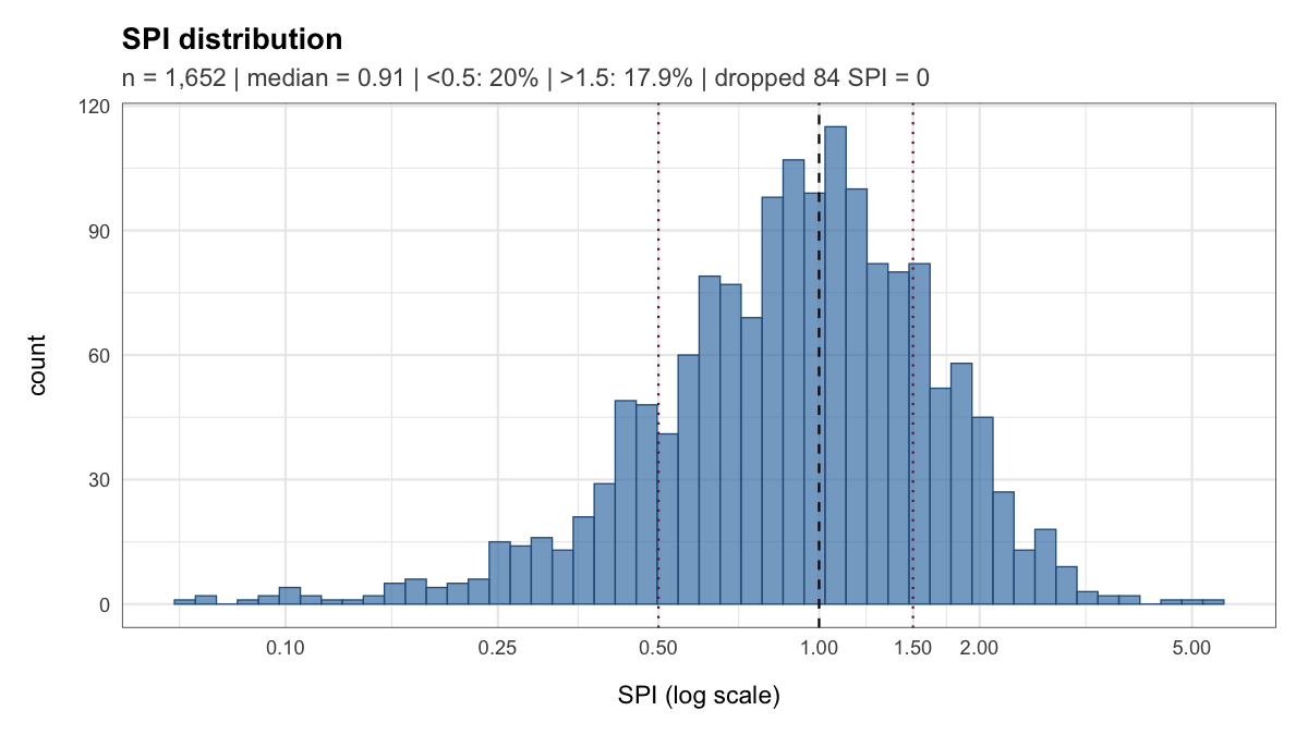
The funnel view plots SPI against the expected count.
Ratios based on small expected counts can vary widely, so inspect them
with their credible intervals. Points are coloured by whether the
district-year met the conventional NPAFP target:
plot(spi_year, type = "funnel")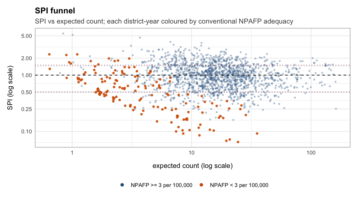
The caterpillar view shows the lowest and highest SPI
values with their credible intervals:
plot(spi_year, type = "caterpillar")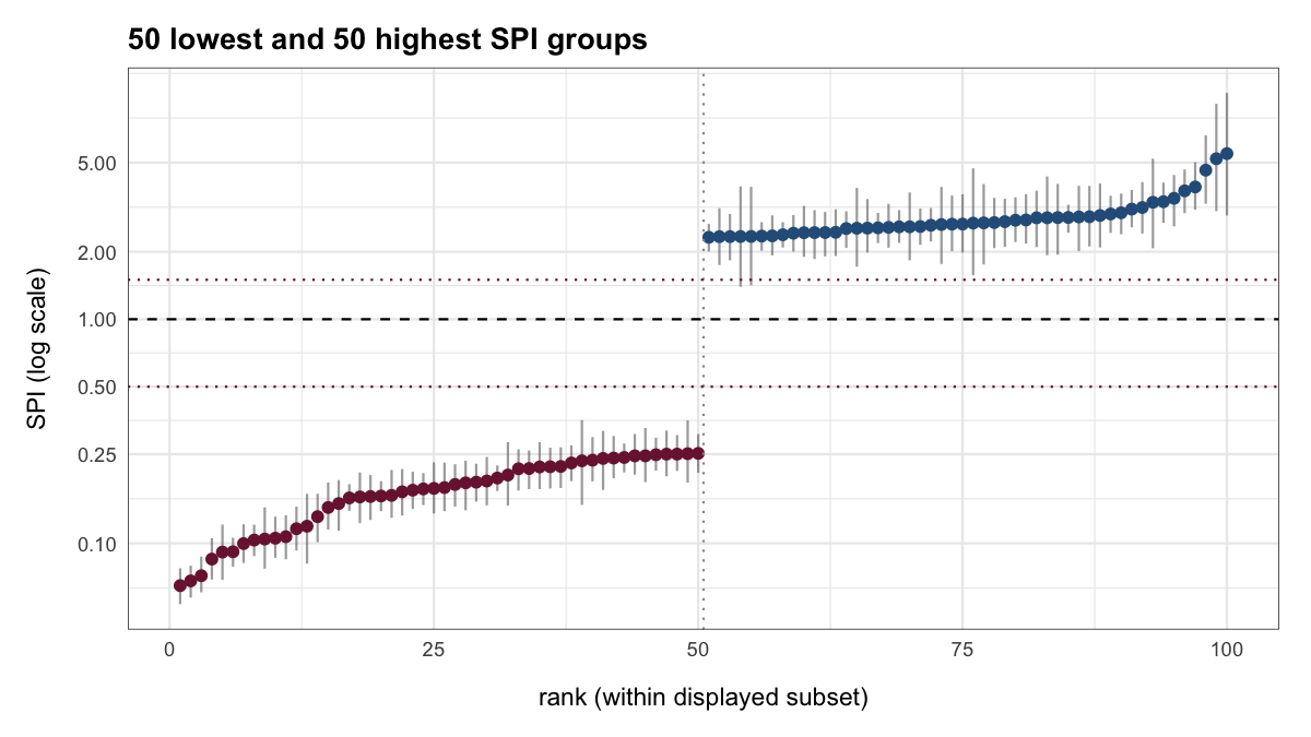
The calibration view compares observed with expected
counts. Points on the diagonal have observed counts equal to their
expected counts:
plot(spi_year, type = "calibration")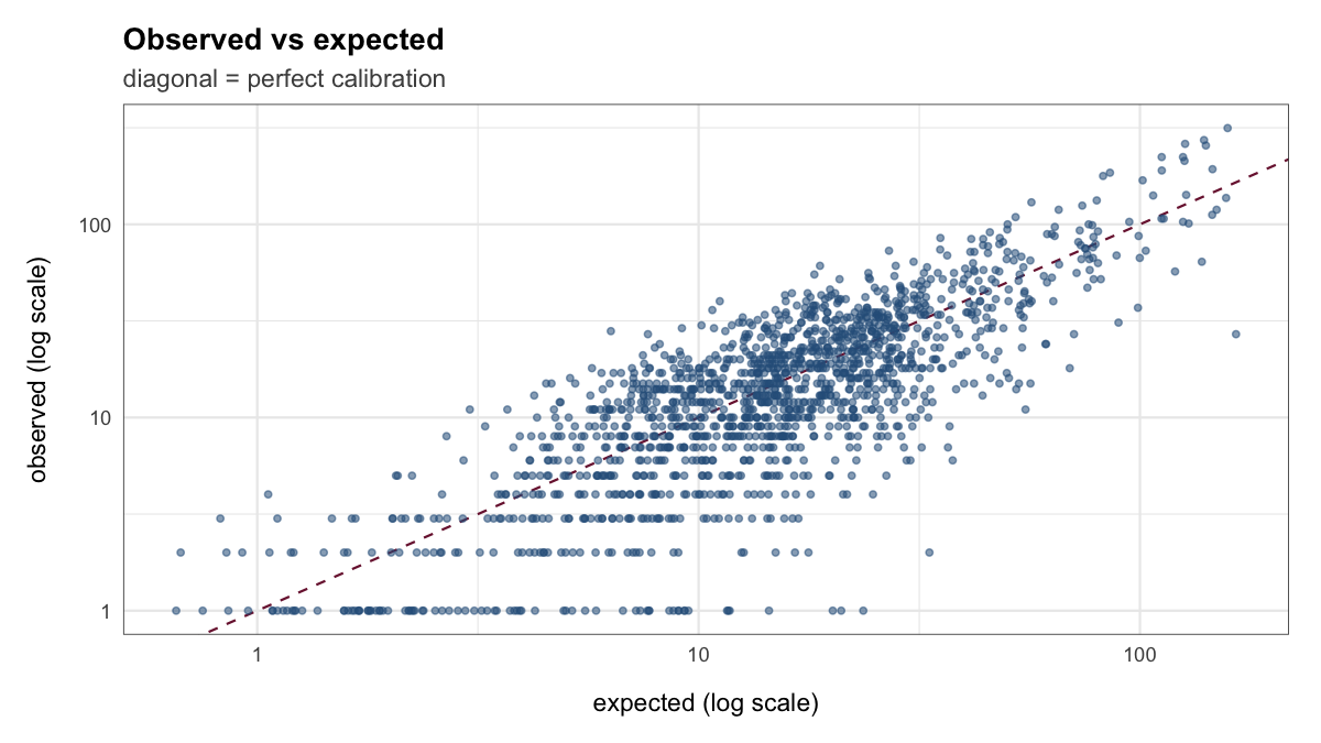
Non-calendar and rolling years
Set year_end_month to use a reporting year other than
January to December. With year_end_month = 4, each
reporting year runs from May to April and is labelled by its ending
year: May 2023 to April 2024 is labelled 2024. Its expected counts are
predicted using data up to April 2023. The first May to April year with
three years of data before it is 2019:
spi_may_apr <- spi_index(
  cases = synth$cases,
  population = synth$population,
  adjacency = synth$boundaries,
  first_assessment = 2019,
  last_assessment = 2024,
  year_end_month = 4,
  id_col = "adm2_guid",
  n_draws = 500,
  seed = 42,
  verbose = FALSE
)

spi_may_apr$windows
#> # A tibble: 6 x 7
#>    year window_start window_end training_start training_end months districts
#>   <int> <date>       <date>     <date>         <date>        <int>     <int>
#> 1  2019 2018-05-01   2019-04-01 2015-01-01     2018-04-01       12       236
#> 2  2020 2019-05-01   2020-04-01 2015-01-01     2019-04-01       12       236
#> 3  2021 2020-05-01   2021-04-01 2015-01-01     2020-04-01       12       236
#> 4  2022 2021-05-01   2022-04-01 2015-01-01     2021-04-01       12       236
#> 5  2023 2022-05-01   2023-04-01 2015-01-01     2022-04-01       12       236
#> 6  2024 2023-05-01   2024-04-01 2015-01-01     2023-04-01       12       236
When the data end before the last year closes, the final assessment
covers fewer than 12 months. spi_index() keeps it with a
warning, and n_months shows how many months each
district-year covers.
For a rolling 12-month SPI that is updated every month, rerun
spi_index() each month with year_end_month set
to the month that has just closed. Each run covers the 12 months ending
in that month and uses earlier months to predict the expected
counts.
Use a consistent model specification, centring setting, and reporting year when comparing years.
Next steps
Interpreting SPI explains how to read these results with the conventional NPAFP rate, timeliness, and stool adequacy. Model options and sensitivity covers covariates, overdispersion, spatial structure and sensitivity checks. Using SPI for district review shows how to compare SPI with the NPAFP target and organise a district review.