How SPI works

SPI compares a district’s current reporting with earlier reporting and the national pattern. It divides reported cases by expected cases, then divides the result by the national ratio for the same period. The simple SPI calculates expected counts from the district’s own earlier rate. The model-based SPI estimates them with a spatial and temporal model. This article explains both calculations and their limitations. For worked examples, see Calculating the simple SPI and Calculating the model-based SPI.

The comparison

For district $i$ and assessment year $t$, let $O_{it}$ be the reported NPAFP count and $E_{it}$ the expected count, estimated from years before $t$ only. The district’s observed-to-expected ratio is $O_{it}/E_{it}$. SPI divides it by the national ratio for the same year:

$$\text{SPI}_{it} = \frac{O_{it}/E_{it}}{r_t}, \qquad r_t = \frac{\sum_j O_{jt}}{\sum_j E_{jt}}$$

An SPI of 1 means the district’s ratio equals the national ratio. The two methods differ in how they calculate $E_{it}$ and which districts they include in the national sums.

	Simple SPI	Model-based SPI
Reporting history	The district’s cases and child-years over all earlier years	Earlier months of all districts, through the fitted model
Population adjustment	Expected count is current population times the earlier rate	Log exposure as an offset, a term whose coefficient is fixed at 1
Information from other districts	None	Partial pooling and a spatial effect, with more influence where a district’s own data provide little information
Seasonality and year effects	None; annual counts only	Harmonic seasonality and an exchangeable year effect
National centring	Always applied	Default; centre = "none" returns the uncentred ratio
Uncertainty	None; one value per district-year	Posterior medians and 90% credible intervals, reflecting uncertainty in expected counts

The simple SPI

spi_simple() calculates the expected count from the district’s own earlier reporting. For district $i$ and assessment year $t$, NPAFP cases and annual under-15 populations are added across all earlier years $s < t$ in the data:

$$Y_i = \sum_{s<t} Y_{is}, \qquad P_i = \sum_{s<t} P_{is}, \qquad r_i = Y_i / P_i$$

Here $P_i$ is earlier exposure in child-years, and all rates in the equations are per child-year. The output tables multiply rates by 100,000 by default. The previous rate $r_i$ is defined only when $P_i > 0$.

History check. A positive expected count can be calculated when the district has at least one earlier year and at least one earlier case. With earlier years but no earlier case ($Y_i = 0$), $r_i = 0$, the expected count is 0, and O/E and SPI are NA; history_check is "no previous case". With no earlier year ($P_i = 0$), $r_i$, the expected count, O/E and SPI are all NA; history_check is "no previous year". Otherwise history_check is "ok". The district’s previous rate is used unchanged.

Index. $E_{it} = P_{it} \, r_i$, calculated as $P_{it} Y_i / P_i$, and

$$\text{SPI}_{it} = \frac{Y_{it}/E_{it}}{\sum_{j:E_{jt}>0} Y_{jt} \big/ \sum_{j:E_{jt}>0} E_{jt}}$$

The national observed-to-expected ratio is calculated from district-years with a positive expected count. Districts with no positive expectation do not contribute to national centring. A zero national ratio gives NA for every district’s SPI, including those with history_check = "ok".

Population check. Each district’s consecutive-year change in log population is compared with the median change across districts in the same year. A change is unusual when its deviation lies outside Tukey’s far-out fences (three interquartile ranges beyond the quartiles) and has absolute magnitude greater than $\log(1.1)$. This is a multiplicative threshold relative to the median growth factor: above 1.1 or below $1/1.1$, rather than a symmetric 10% change in population. Fences are calculated from all available consecutive-year deviations; fewer than four deviations give no change flags.

For each assessment year, the check considers the district’s population records up to that year. population_qc is check_spike when an unusual deviation is followed by an unusual deviation in the opposite direction among the next two recorded transitions, check_change for any other unusual deviation, check_history when population records do not cover all dataset years up to that year, and ok otherwise. These labels take precedence in that order. With a complete annual series, the two transitions cover two years; gaps can extend that interval. The check does not alter populations.

The model-based SPI

spi_index() estimates expected counts with the model below. It fits the model for each assessment year using preceding years only, so the year being assessed does not contribute to its own expectation. In the accompanying study, each district’s earlier reporting provided most of the basis for its expected counts. Information from other districts contributed more when the district’s own history provided little information.

Model specification

With annual population data, the default model without covariates estimates expected counts for each district $i$ and month $t$:

$$Y_{it} \sim \text{NegBin}(\mu_{it}, \kappa)$$

$$\log \mu_{it} = \log(P_{it}/12) + \beta_0 + f(\text{month}_t) + \gamma_{y(t)} + b_i$$

where

• $P_{it}$ is the district’s annual under-15 population for the year containing month $t$; $P_{it}/12$ approximates that month’s exposure in child-years
• $\beta_0$ is the background log rate; $\exp(\beta_0)$ is the rate per child-year when the other terms are zero
• $f(\text{month}_t)$ is harmonic seasonality (12- and 6-month periodicity)
• $\gamma_{y(t)}$ is an exchangeable year effect
• $b_i$ is a BYM2 spatial random effect (Riebler et al. 2016)
• $\kappa > 0$ is the negative binomial size parameter, with $\operatorname{Var}(Y_{it}\mid\mu_{it},\kappa) = \mu_{it} + \mu_{it}^2/\kappa$; larger values approach the Poisson model

The INLA BYM2 parameterisation is

$$b_i = \frac{1}{\sqrt{\tau_b}}\left(\sqrt{\phi}\,u_i^* + \sqrt{1-\phi}\,v_i\right),$$

where $u_i^*$ is the scaled, spatially structured effect and $v_i$ is an independent standard normal effect. The precision $\tau_b$ controls the overall scale and $\phi\in[0,1]$ controls the balance between the two components. The package applies scaling and constraints separately to disconnected components of the adjacency graph.

The negative binomial parameterisation above is the default overdispersion = "nb". If population data are supplied by month, the package instead uses log(pop) directly: those values must already represent monthly exposure in child-years.

Optional covariates add $x_{it}^{\top}\beta$ to the linear predictor. They are not part of the default SPI used in the accompanying study.

overdispersion = "iid" uses a Poisson model with an independent normal observation-level term $\epsilon_{it}$ in the linear predictor. "none" fits a Poisson model without that extra term. Use spi_compare_overdispersion() to compare the three options.

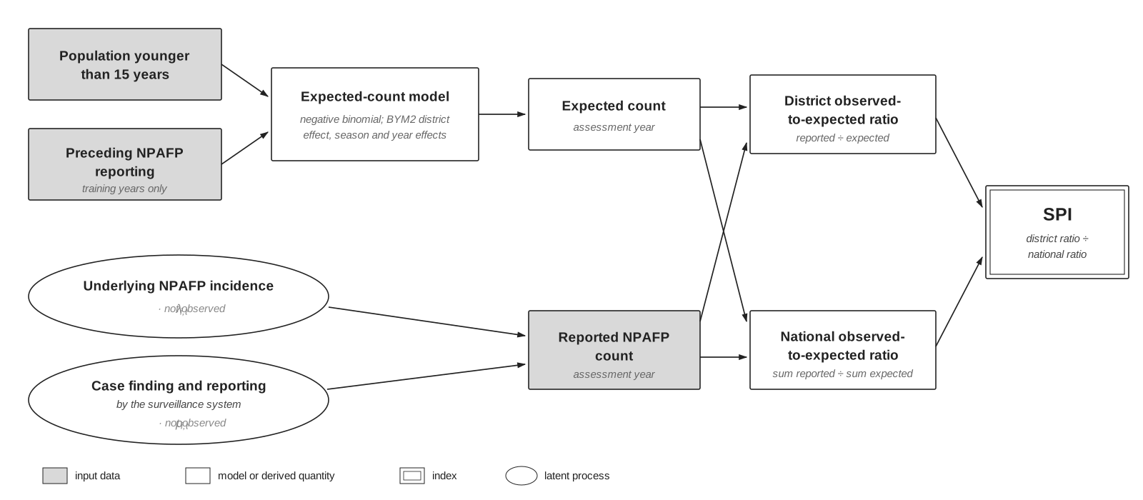
Reported counts reflect both underlying NPAFP incidence and surveillance reporting. spi_index() estimates each year’s expected counts from preceding years only.

National centring and uncertainty

For district $i$ and year $y$, let $O_{iy}$ be the annual observed count. Within each posterior draw $s$, sum the monthly expected counts first:

$$E_{iy}^{(s)} = \sum_{t:\,y(t)=y}\mu_{it}^{(s)}, \qquad \widetilde E_{iy} = \operatorname{median}_s E_{iy}^{(s)}.$$

The annual median is therefore taken after summing months. The default index is calculated for each draw as

$$\text{SPI}_{iy}^{(s)} = \frac{O_{iy}/E_{iy}^{(s)}}{r_y^{(s)}}, \qquad r_y^{(s)} = \frac{\sum_i O_{iy}}{\sum_i E_{iy}^{(s)}}$$

The national ratio is calculated within the same draw as the district ratio. Uncertainty shared by every district in a year, such as a common year effect, therefore cancels before the medians and credible intervals are taken. Within each draw, the expected-count-weighted mean of the centred index is exactly 1. SPI medians and credible intervals summarise the centred draws. They reflect uncertainty in the expected counts, conditional on observed counts, and do not include extra variation from simulated future counts. spi_dy$national reports $\sum_i O_{iy}$ divided by the median of $\sum_i E_{iy}^{(s)}$. In particular, zero observed cases give zero SPI in every draw when the expected counts and national ratio are positive.

National sums include rows with finite observed counts and finite, positive expected counts. A year with no observed cases nationally has an undefined centred SPI, returned as NA. centre = "none" returns the uncentred observed-to-expected ratio.

Limitations

These limits follow from how the reference is estimated and how the ratio is centred:

Limitation	What to check
Persistent low reporting can become the baseline	A district with years of low reporting can have an SPI near 1. Keep the conventional NPAFP target as an external benchmark; persistent failure to meet it remains a reason for closer review.
National change is removed when centre = "national"	Review the national observed-to-expected ratio in spi_dy$national separately. SPI describes relative district differences, so a shared decline can leave district SPI values largely unchanged. Also inspect absolute reporting rates and counts.
Population and boundary errors affect the comparison	Population error affects both expected counts and the conventional rate. Check denominators and use consistent boundaries across years, especially after district splits or mergers.
Simple SPI can be unstable with little history	The earlier rate is used unchanged, even when based on a single case. Review earlier years, cases and child-years. With no earlier case or year, SPI is unavailable.
Model-based estimates use more information from other districts when history is limited	Sparse reporting histories give the model less district-specific information. Review the available history and uncertainty before interpreting changes.
Using neighbours in the model can reduce estimated differences between districts	Sharing information improves stability but can pull an unusual district towards its neighbours. Check local counts and context when the fitted expectation seems implausible.
Results depend on model choices	The training period, spatial structure, seasonality, priors, and centring affect results. Keep these choices consistent when comparing years and assess sensitivity to plausible alternatives.

SPI does not directly estimate missed cases, detection probability, poliovirus circulation, outbreak risk, or overall surveillance quality.