The STEPS field guide combines SPI with timeliness, stool adequacy,
and findings from nearby districts and earlier years. It works with the
simple SPI and the model-based SPI. The examples below use synthetic
data and the model-based SPI from spi_index(). With the simple SPI explains how the
review rules differ for spi_simple() results.
- Calculate SPI and compare it with the NPAFP target. SPI uses only case counts and population.
- Prepare counts for specimen transport and stool adequacy that supply timeliness and stool adequacy.
- Run the STEPS field guide, which combines SPI with those counts through the five STEPS components.
- Read the review labels.
- If needed, change the SPI cutoff or the classification rule.
- To use the simple SPI instead, see With the simple SPI.
- Produce a field guide table or a one-page district report.
From SPI to review
The field guide starts from a spi_compare_npafp()
result, which classifies each district-year by its SPI and the
conventional NPAFP target. This code calculates annual and monthly SPI
and builds that comparison. Calculating the
model-based SPI explains the first two steps.
library(spi)
synth <- synth_surveillance
adj <- spi_adjacency(synth$boundaries, id_col = "adm2_guid")

spi_year <- spi_index(
  cases = synth$cases,
  population = synth$population,
  adjacency = adj,
  first_assessment = 2018,
  id_col = "adm2_guid",
  n_draws = 500,
  seed = 42,
  verbose = FALSE
)
spi_month <- spi_index(
  cases = synth$cases,
  population = synth$population,
  adjacency = adj,
  first_assessment = 2018,
  level = "district_month",
  id_col = "adm2_guid",
  n_draws = 500,
  seed = 42,
  verbose = FALSE
)
Compare each district-year’s SPI with the NPAFP target used here: 3
non-polio AFP cases per 100,000 under-15 person-years, matching the
study definition. Programmes should use the target that applies in their
setting. The four categories show where the two measures agree or
differ. The "SPI below threshold only" category identifies
districts that meet the NPAFP target but have an SPI below 1.
comparison <- spi_compare_npafp(
  spi = spi_year,
  cases = synth$cases,
  population = synth$population,
  boundaries = synth$boundaries,
  spi_threshold = 1,
  spi_rule = "median",
  npafp_target = 3,
  verbose = FALSE
)
Count the district-years in each category:
comparison$district_year |>
  dplyr::count(category, name = "district_years", .drop = FALSE)
#> # A tibble: 4 x 2
#>   category                 district_years
#>   <fct>                             <int>
#> 1 Neither below                       691
#> 2 SPI below threshold only            730
#> 3 NPAFP below target only              29
#> 4 Both below                          202
Three panels for one year show the conventional NPAFP rate, the posterior median SPI, and the SPI and NPAFP category of each district:
spi_compare_npafp_maps(comparison, boundaries = synth$boundaries, year = 2023)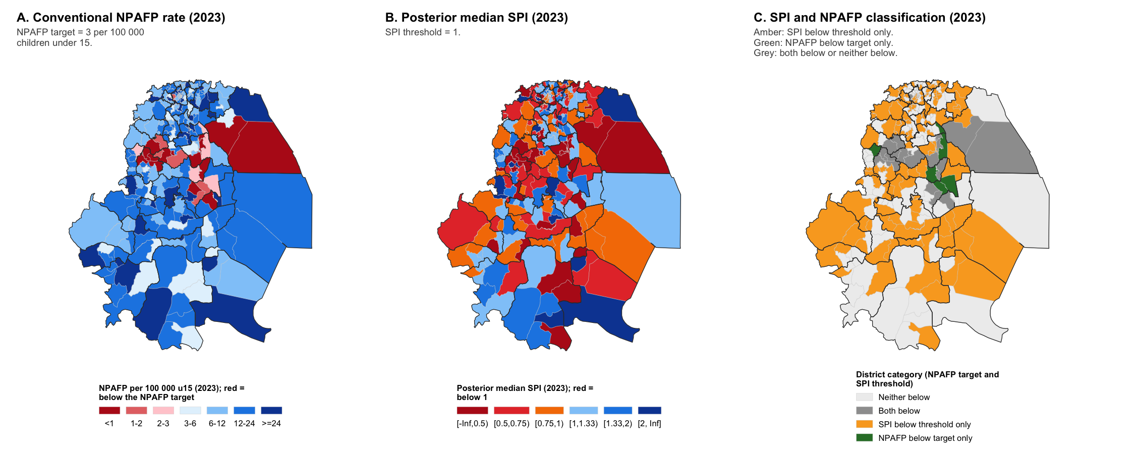
The five STEPS components
spi_field_guide() uses five STEPS components to review
districts with a low SPI. Strength describes the size and uncertainty of
the shortfall; extent and persistence show whether it is also seen in
the wider area or the previous year. Timeliness and stool adequacy
describe specimen handling:
| Letter | Component | What it asks |
|---|---|---|
| S | Strength | How large is the shortfall, and does the 90% credible interval lie entirely below the reference value of 1? |
| T | Timeliness | Are specimens reaching the laboratory within 3 days? |
| E | Extent | Is an SPI below the chosen cutoff more common among other districts in the same area than nationally? |
| P | Persistence | Was SPI also below the chosen cutoff in the previous year? |
| S | Stool adequacy | Were two adequate stool specimens collected? |
The five STEPS components are reported separately. The review label depends on strength, extent, and persistence. Timeliness and stool adequacy help the reviewer assess specimen handling but do not change that label. The timeliness component uses specimen transport only, not notification or investigation timeliness.
Prepare process data
The field guide calculates timeliness and stool adequacy from the
counts supplied through process, with one row per district
and year. These counts do not change SPI. synth$afp_process
contains the required columns:
head(synth$afp_process)
#> # A tibble: 6 x 6
#>   adm2_guid               year n_cases n_adequate n_transport n_transport_timely
#>   <chr>                  <int>   <int>      <int>       <int>              <int>
#> 1 {01325AA0-BEA1-66FE-9~  2015       1          1           1                  0
#> 2 {01325AA0-BEA1-66FE-9~  2016       2          2           2                  2
#> 3 {01325AA0-BEA1-66FE-9~  2017       0          0           0                  0
#> 4 {01325AA0-BEA1-66FE-9~  2018       2          1           2                  1
#> 5 {01325AA0-BEA1-66FE-9~  2019       5          4           5                  3
#> 6 {01325AA0-BEA1-66FE-9~  2020       2          2           2                  2
n_cases is the number of AFP cases and
n_adequate the number with adequate stool specimens.
n_transport is the number of cases with both a second stool
collection date and a laboratory receipt date, and
n_transport_timely is the number of those received by the
laboratory within 3 days. A component raises concern when its percentage
is below process_target (80 by default), and it is not
assessed when the district has fewer than process_min_cases
cases (5 by default).
Run the field guide
Supply AFP process counts through process. Optional
adjacency, spi_month, detections,
and es inputs add neighbouring-district, seasonal, and
poliovirus detection context; they do not change the review label.
# optional AFP poliovirus detection records, used only as supporting context
detections <- synth$virus_outcome |>
  dplyr::filter(any_virus == 1) |>
  dplyr::select(adm2_guid, year)

fg <- spi_field_guide(
  comparison = comparison,
  # AFP process counts: the timeliness (T) and stool adequacy (S) components
  process = synth$afp_process,
  # context only; these do not change the review label
  adjacency = adj,
  spi_month = spi_month,
  detections = detections,
  es = synth$es_district_year,
  es_col = "n_positive",
  spi_cut = 1,
  verbose = FALSE
)

fg
#> # A tibble: 3 x 3
#>   verdict                 n   pct
#>   <chr>               <int> <dbl>
#> 1 Priority for review    86  36.4
#> 2 Monitor                57  24.2
#> 3 No SPI indication      93  39.4
#> # A tibble: 86 x 11
#>    district   obs   exp   spi cri       npafp extent persist transport adequacy
#>    <chr>    <int> <dbl> <dbl> <chr>     <dbl> <lgl>  <lgl>       <dbl>    <dbl>
#>  1 Khandor      0   2.2   0   0.00-0.00   0   TRUE   TRUE           NA       NA
#>  2 Vasheth      0   0.7   0   0.00-0.00   0   TRUE   FALSE          NA       NA
#>  3 Arddor       0   1.6   0   0.00-0.00   0   TRUE   TRUE           NA       NA
#>  4 Ardor        0   1.1   0   0.00-0.00   0   TRUE   TRUE           NA       NA
#>  5 Doloth       0   1.1   0   0.00-0.00   0   TRUE   TRUE           NA       NA
#>  6 Raenan       0   1     0   0.00-0.00   0   TRUE   TRUE           NA       NA
#>  7 Chakis       0   1.7   0   0.00-0.00   0   TRUE   TRUE           NA       NA
#>  8 Vashoth      0   2.2   0   0.00-0.00   0   TRUE   TRUE           NA       NA
#>  9 Nentha       2  14.9   0.1 0.09-0.12   2   TRUE   FALSE         100      100
#> 10 Suzil        1   7.7   0.1 0.08-0.12   1.6 TRUE   TRUE          100      100
#> # i 76 more rows
#> # i 1 more variable: verdict <chr>
The result reports percentages for timely transport and adequate specimens, plus flags showing whether each is below the chosen target. For the first districts in the latest year:
fg$focal |>
  dplyr::select(
    adm2_name, verdict, n_cases,
    pct_transport_timely, timeliness_concern,
    pct_adequate, adequacy_concern
  ) |>
  dplyr::slice_head(n = 6)
#> # A tibble: 6 x 7
#>   adm2_name verdict n_cases pct_transport_timely timeliness_concern pct_adequate
#>   <chr>     <fct>     <int>                <dbl> <lgl>                     <dbl>
#> 1 Khandor   Priori~       0                 NA   NA                         NA
#> 2 Yolar     No SPI~      12                 66.7 TRUE                       91.7
#> 3 Ostan     No SPI~      43                 66.7 TRUE                       79.1
#> 4 Hartha    Monitor      68                 97.0 FALSE                      88.2
#> 5 Munis     Priori~       1                100   NA                        100
#> 6 Zimmar    No SPI~      15                 80   FALSE                      60
#> # i 1 more variable: adequacy_concern <lgl>
Review labels
The field guide generates three review labels:
- Priority for review: the SPI is below the cutoff, its 90% interval is entirely below 1, and extent or persistence raises concern.
-
Monitor: the SPI is below the cutoff, but the
conditions for
Priority for revieware not all met. - No SPI indication: the SPI is at or above the cutoff. Routine surveillance and review based on other indicators continue.
The meaning of No SPI indication depends on the SPI
rule. Under the default median rule, it means the SPI median is at or
above the cutoff. Under the interval rule, described below, it also
includes district-years whose 90% interval includes 1.
These labels help decide which districts to review first. They do not establish surveillance quality or prescribe a field response.
summary(fg) reports how often each STEPS component
raises concern. spi_field_guide_help() explains the
components and four worked examples in the console.
Changing spi_cut
Set spi_cut to 0.80, 0.60, or
0.40 to focus on progressively larger relative shortfalls.
These cutoffs select districts for review; they have not been validated
as thresholds for taking action.
| Chosen SPI cutoff | Districts included | Interpretation with national centring |
|---|---|---|
1.00 (package default) |
SPI below 1 | District O:E below national O:E |
0.80 |
SPI below 0.80 | District O:E >20% below national O:E |
0.60 |
SPI below 0.60 | District O:E >40% below national O:E |
0.40 |
SPI below 0.40 | District O:E >60% below national O:E |
This table assumes centre = "national", the default.
With centre = "none", the same cutoffs apply to the
uncentred district O:E. These cutoffs help focus review; they are not
validated boundaries between adequate and inadequate surveillance.
Continue to review concerns from timeliness, stool adequacy, or other
indicators even when a district is above the chosen SPI cutoff.
Changing spi_cut changes which district-years enter
review and how extent and persistence are assessed. The strength check
still compares the 90% credible interval with 1. To use the same cutoff
in the comparison, also set spi_threshold in
spi_compare_npafp(). Record the cutoff with the
results.
The labels for the latest year at three cutoffs show the effect. The context inputs do not affect the label, so they are left out here:
label_counts <- function(comparison, cut = 1) {
  guide <- spi_field_guide(
    comparison = comparison,
    process = synth$afp_process,
    spi_cut = cut,
    verbose = FALSE
  )

  dplyr::count(guide$focal, verdict, name = "district_years")
}

purrr::map(c(1, 0.8, 0.6), function(cut) {
  label_counts(comparison, cut) |>
    dplyr::mutate(spi_cut = cut)
}) |>
  purrr::list_rbind() |>
  dplyr::arrange(dplyr::desc(spi_cut), verdict)
#> # A tibble: 9 x 3
#>   verdict             district_years spi_cut
#>   <fct>                        <int>   <dbl>
#> 1 Priority for review             86     1
#> 2 Monitor                         57     1
#> 3 No SPI indication               93     1
#> 4 Priority for review             60     0.8
#> 5 Monitor                         31     0.8
#> 6 No SPI indication              145     0.8
#> 7 Priority for review             37     0.6
#> 8 Monitor                         18     0.6
#> 9 No SPI indication              181     0.6
Changing the classification rule
spi_rule decides which district-years count as having an
SPI below the threshold:
-
spi_rule = "median", the default inspi_compare_npafp(), usesspi_medianalone. -
spi_rule = "interval"also requires the upper bound of the 90% credible interval,spi_q95, to be below 1.
spi_field_guide() takes the rule from the comparison
unless its own spi_rule argument is set. Under the interval
rule, a district-year whose interval includes 1 receives
No SPI indication rather than Monitor. Extent
and persistence still use the median. Record the rule with the
results.
comparison_interval <- spi_compare_npafp(
  spi = spi_year,
  cases = synth$cases,
  population = synth$population,
  boundaries = synth$boundaries,
  spi_threshold = 1,
  spi_rule = "interval",
  npafp_target = 3,
  verbose = FALSE
)

dplyr::bind_rows(
  median = dplyr::count(comparison$district_year, category, .drop = FALSE),
  interval = dplyr::count(
    comparison_interval$district_year, category, .drop = FALSE
  ),
  .id = "spi_rule"
)
#> # A tibble: 8 x 3
#>   spi_rule category                     n
#>   <chr>    <fct>                    <int>
#> 1 median   Neither below              691
#> 2 median   SPI below threshold only   730
#> 3 median   NPAFP below target only     29
#> 4 median   Both below                 202
#> 5 interval Neither below              896
#> 6 interval SPI below threshold only   525
#> 7 interval NPAFP below target only     52
#> 8 interval Both below                 179

dplyr::bind_rows(
  median = label_counts(comparison),
  interval = label_counts(comparison_interval),
  .id = "spi_rule"
)
#> # A tibble: 6 x 3
#>   spi_rule verdict             district_years
#>   <chr>    <fct>                        <int>
#> 1 median   Priority for review             86
#> 2 median   Monitor                         57
#> 3 median   No SPI indication               93
#> 4 interval Priority for review             86
#> 5 interval Monitor                         21
#> 6 interval No SPI indication              129
With the simple SPI
Pass a spi_simple() result to
spi_compare_npafp(), then pass the comparison to
spi_field_guide(). The simple SPI has no credible interval,
so the strength component uses the SPI value alone. The default cutoff
is spi_cut = 0.5. A district-year below this cutoff is
labelled Priority for review when extent or persistence
also raises concern, or Monitor when neither does. The
cutoff selects larger relative shortfalls; it does not measure
uncertainty.
annual <- synth$cases |>
  dplyr::mutate(year = as.integer(format(month, "%Y"))) |>
  dplyr::summarise(count = sum(count), .by = c(adm2_guid, year))

spi_simple_year <- spi_simple(
  data = annual,
  population = synth$population,
  id_col = "adm2_guid",
  count_col = "count",
  pop_col = "pop_u15",
  first_assessment = 2018,
  verbose = FALSE
)

comparison_simple <- spi_compare_npafp(
  spi = spi_simple_year,
  boundaries = synth$boundaries,
  npafp_target = 3,
  verbose = FALSE
)

dplyr::bind_rows(
  model = label_counts(comparison),
  simple = label_counts(comparison_simple, cut = 0.5),
  .id = "spi"
)
#> # A tibble: 6 x 3
#>   spi    verdict             district_years
#>   <chr>  <fct>                        <int>
#> 1 model  Priority for review             86
#> 2 model  Monitor                         57
#> 3 model  No SPI indication               93
#> 4 simple Priority for review             25
#> 5 simple Monitor                         16
#> 6 simple No SPI indication              195
Set spi_cut to choose a different cutoff for the simple
SPI. Seasonal context needs monthly model-based SPI results
(spi_month), so it is not available from the simple SPI
alone.
Field guide table
Use spi_field_guide_table() to create a gt
or flextable report. layout = "worked" puts
the STEPS components in rows and selects four districts with different
findings; layout = "scan" puts districts in rows for
scanning a longer list. Cells are coloured by level of concern. The
illustration below uses the bundled synth_field_guide
example.
spi_field_guide_table(fg, engine = "gt", layout = "worked")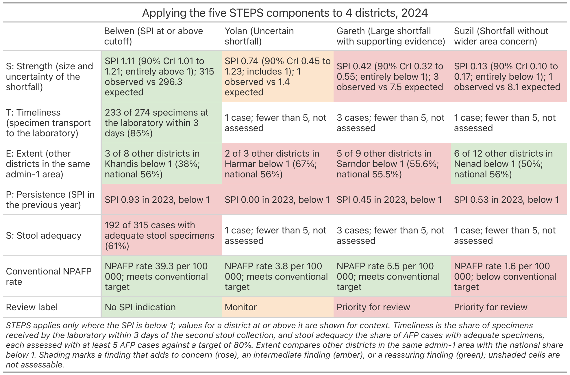
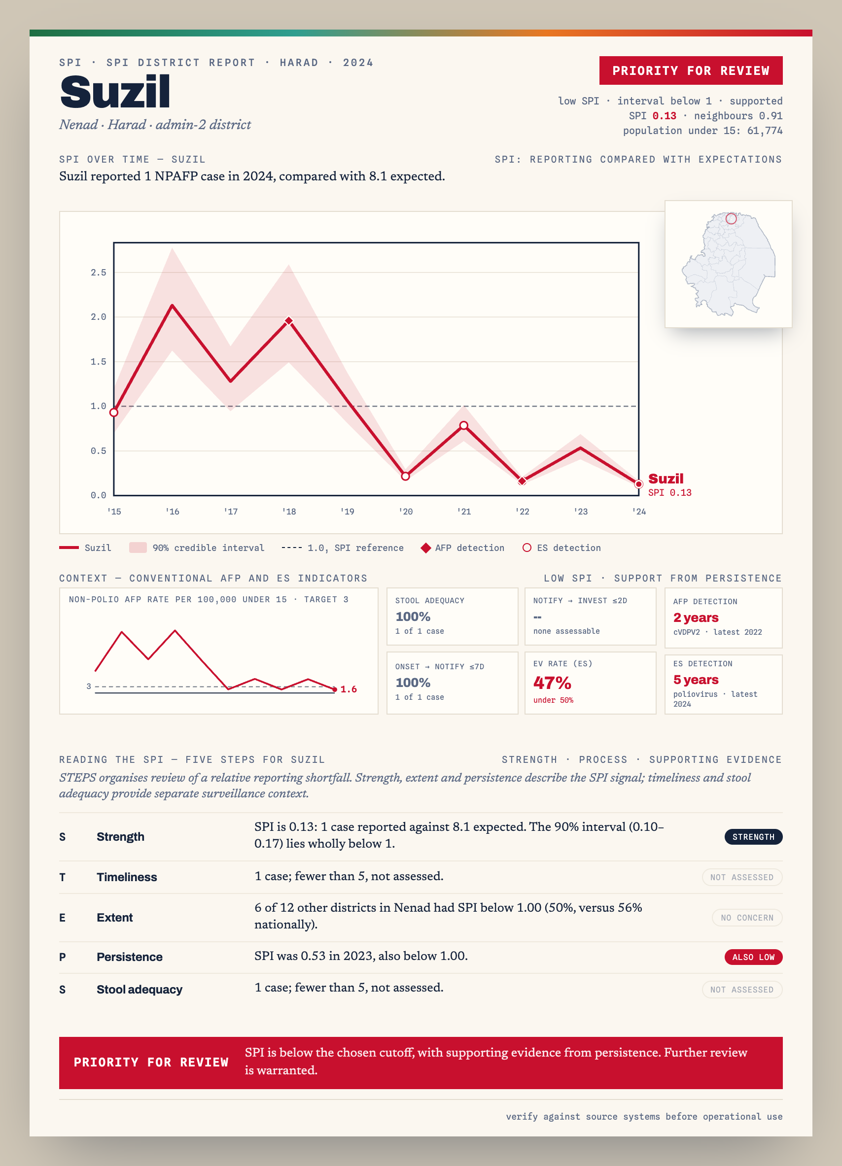
District report
Create an A4 report for one district, with its SPI trend, map, STEPS
findings, and detection context. Pass indicators_df to add
the NPAFP rate over time and summary boxes for stool adequacy,
timeliness, and the enterovirus (EV) isolation rate from environmental
samples. The example simulates the notification-to-investigation and EV
figures. Set path to save HTML and PNG files:
source(system.file("examples", "pager_indicators.R", package = "spi"))
indicators <- example_indicators(fg)

spi_field_guide_pager(
  fg, district = "Tirwen", boundaries = synth$boundaries,
  id_col = "adm2_guid", indicators_df = indicators, path = "reports/"
)
The report below uses the bundled synth_field_guide
example. It shows the district with the lowest non-zero SPI among those
labelled Priority for review in the latest year: